Reference Input Data Library (RIPL)

In this brief notebook, we use the processed RIPL data to explore and visualize some attributes. Let us start by importing the necessary packages.

NOTE: This notebook is not meant to be a complete exploration resource. You are responsible for exploring and validating any provided data.

# # PROTOTYPE
# import sys
# sys.path.append("../..")

import pandas as pd
import numpy as np
pd.set_option('display.max_columns', 500)
pd.set_option('display.max_rows', 50)

import seaborn as sns
import matplotlib.pyplot as plt
import os

import nucml.datasets as nuc_data

# Specifying directory to save figures
figure_dir = "Figures/"

Loading RIPL/ENSDF Data

Let us first load both the original and the cut-off RIPL data. Recall that the cut-off version is based on the RIPL cut-off parameters.

ensdf_df = nuc_data.load_ensdf(append_ame=True)
ensdf_cutoff_df = nuc_data.load_ensdf(cutoff=True, append_ame=True)

INFO:root:Reading data from C:/Users/Pedro/Desktop/ML_Nuclear_Data/ENSDF\CSV_Files/ensdf.csv
INFO:root:AME: Reading and loading Atomic Mass Evaluation files from:
 C:/Users/Pedro/Desktop/ML_Nuclear_Data/AME/CSV_Files\AME_all_merged_no_NaN.csv
INFO:root:Reading data from C:/Users/Pedro/Desktop/ML_Nuclear_Data/ENSDF\CSV_Files/ensdf_cutoff.csv
INFO:root:AME: Reading and loading Atomic Mass Evaluation files from:
 C:/Users/Pedro/Desktop/ML_Nuclear_Data/AME/CSV_Files\AME_all_merged_no_NaN.csv

Plotting Some Features Distributions

Isotope Energy Distribution

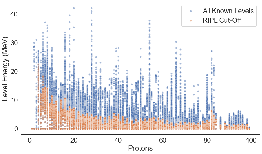
Let us observe what is the energy distribution as a function of the number of protons for all known levels against the cut-off dataset.

sns.set(font_scale = 2)
sns.set_style("white")

plt.figure(figsize=(14, 8))
sns.scatterplot(ensdf_df.Z, ensdf_df.Energy, alpha=0.5, label="All Known Levels")
sns.scatterplot(ensdf_cutoff_df.Z, ensdf_cutoff_df.Energy, alpha=0.5, label="RIPL Cut-Off")
plt.ylabel("Level Energy (MeV)")
plt.xlabel("Protons")
plt.savefig(os.path.join(figure_dir, 'ENSDF_Z_E.png'), transparent=False, bbox_inches='tight', dpi=600)

C:\Users\Pedro\Anaconda3\envs\nucml\lib\site-packages\seaborn\_decorators.py:36: FutureWarning: Pass the following variables as keyword args: x, y. From version 0.12, the only valid positional argument will be `data`, and passing other arguments without an explicit keyword will result in an error or misinterpretation.
  warnings.warn(
C:\Users\Pedro\Anaconda3\envs\nucml\lib\site-packages\seaborn\_decorators.py:36: FutureWarning: Pass the following variables as keyword args: x, y. From version 0.12, the only valid positional argument will be `data`, and passing other arguments without an explicit keyword will result in an error or misinterpretation.
  warnings.warn(

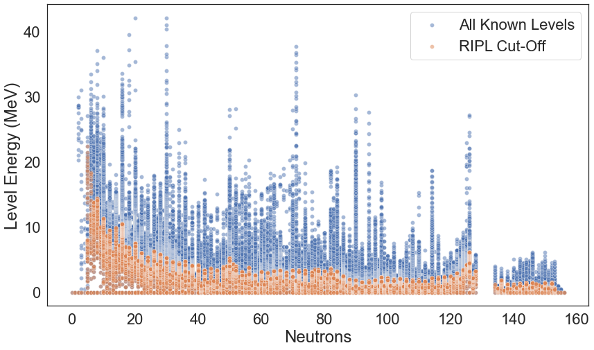
Similarly, for neutrons:

plt.figure(figsize=(14, 8))
sns.scatterplot(ensdf_df.N, ensdf_df.Energy, alpha=0.5, label="All Known Levels")
sns.scatterplot(ensdf_cutoff_df.N, ensdf_cutoff_df.Energy, alpha=0.5, label="RIPL Cut-Off")
plt.ylabel("Level Energy (MeV)")
plt.xlabel("Neutrons")
plt.savefig(os.path.join(figure_dir, 'ENSDF_N_E.png'), transparent=False, bbox_inches='tight', dpi=600)

C:\Users\Pedro\Anaconda3\envs\nucml\lib\site-packages\seaborn\_decorators.py:36: FutureWarning: Pass the following variables as keyword args: x, y. From version 0.12, the only valid positional argument will be `data`, and passing other arguments without an explicit keyword will result in an error or misinterpretation.
  warnings.warn(
C:\Users\Pedro\Anaconda3\envs\nucml\lib\site-packages\seaborn\_decorators.py:36: FutureWarning: Pass the following variables as keyword args: x, y. From version 0.12, the only valid positional argument will be `data`, and passing other arguments without an explicit keyword will result in an error or misinterpretation.
  warnings.warn(

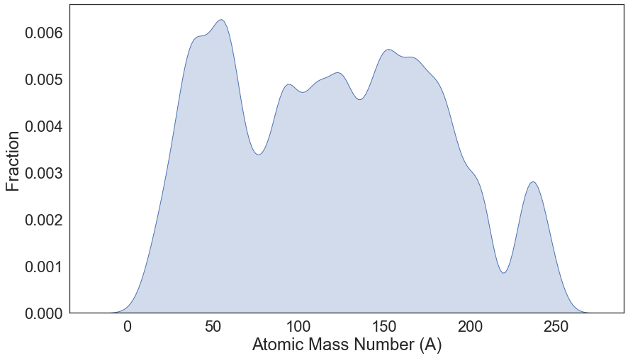
Atomic Mass Number Distribution

plt.figure(figsize=(14,8))
g = sns.kdeplot(ensdf_df.A, shade=True);
g.set(xlabel="Atomic Mass Number (A)", ylabel="Fraction")
plt.savefig(os.path.join(figure_dir, 'ENSDF_Atomic_Mass_Dist.png'), bbox_inches='tight', dpi=600)

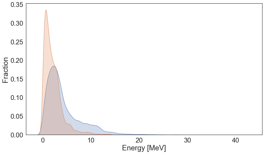
Energy Distribution

plt.figure(figsize=(14, 8))
sns.kdeplot(ensdf_df.Energy.values, shade=True, label="All Known Levels");
sns.kdeplot(ensdf_cutoff_df.Energy.values, shade=True, label='RIPL Cut-Off');
plt.xlabel("Energy [MeV]")
plt.ylabel("Fraction")
plt.savefig(os.path.join(figure_dir, 'ENSDF_E_Dist.png'), bbox_inches='tight', dpi=600)

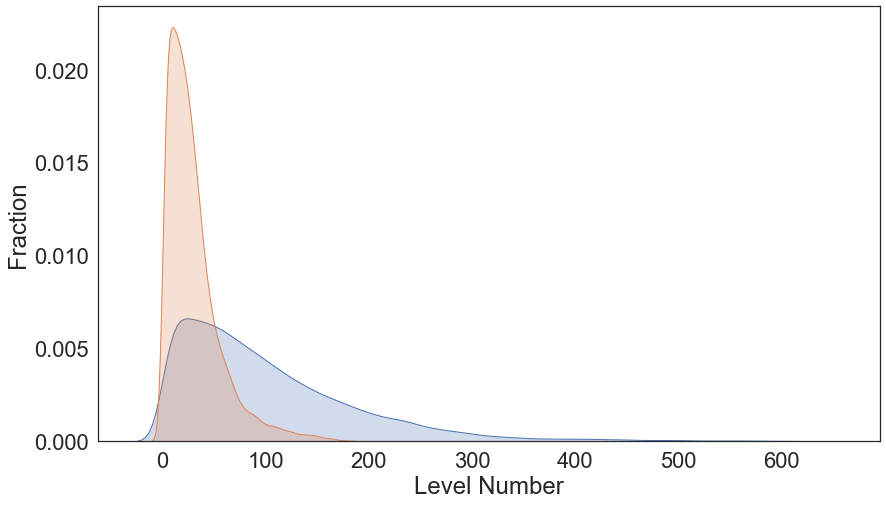
Level Number Distribution

plt.figure(figsize=(14,8))
sns.kdeplot(ensdf_df.Level_Number.values, shade=True, label="All Known Levels");
sns.kdeplot(ensdf_cutoff_df.Level_Number.values, shade=True, label="RIPL Cut-Off");
plt.xlabel("Level Number")
plt.ylabel("Fraction")
plt.savefig(os.path.join(figure_dir, 'ENSDF_L_Dist.png'), bbox_inches='tight', dpi=600)

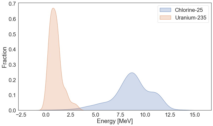
Uranium and Chlorine Energy Distribution

plt.figure(figsize=(14, 8))
chlorine = ensdf_df[ensdf_df.Element_w_A == "35Cl"]
uranium = ensdf_df[ensdf_df.Element_w_A == "233U"]
sns.kdeplot(chlorine.Energy.values, shade=True, label="Chlorine-25");
sns.kdeplot(uranium.Energy.values, shade=True, label='Uranium-235');
plt.xlabel("Energy [MeV]")
plt.ylabel("Fraction")
plt.legend()
plt.savefig(os.path.join(figure_dir, 'ENSDF_Cl_U_E_Dist.png'), bbox_inches='tight', dpi=600)

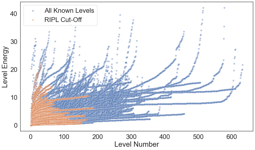
Energy vs Level Number

Ideally, we would like to model the level energy vs level number. It is a difficult challenge as there are collective states and more. Furthemore, when implementing the RIPL cut-off parameters, we lose more than half of the avaliable data for training.

plt.figure(figsize=(14, 8))
sns.scatterplot(x='Level_Number', y='Energy', data=ensdf_df, alpha=0.4, label="All Known Levels")
sns.scatterplot(x='Level_Number', y='Energy', data=ensdf_cutoff_df, alpha=0.4, label="RIPL Cut-Off")
plt.xlabel("Level Number")
plt.ylabel("Level Energy")
plt.savefig(os.path.join(figure_dir, 'ENSDF_E_vs_L.png'), bbox_inches='tight', dpi=600)

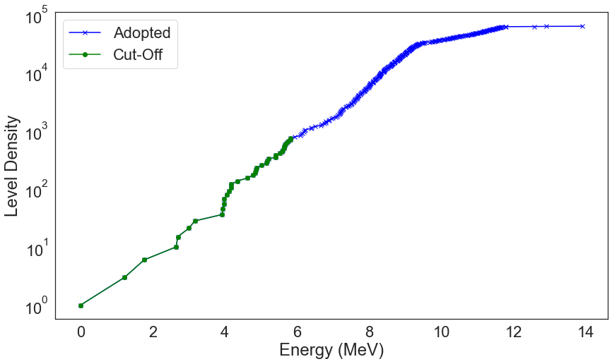
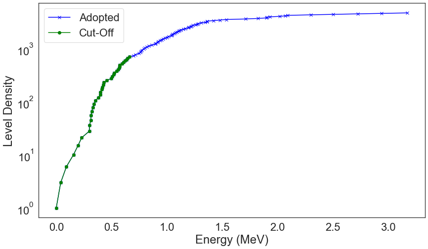
NucML Plotting Utilities: Level and Level Density

For EXFOR, a useful future might be the level density at incident energies. To model RIPL/XUNDL we can take two approaches: (1) model the level energy as a function of the level number with the cut-off dataset or (2) model the level density. We can visualize the level density using NucML ensdf plotting utilities. Let us import it.

import nucml.ensdf.plot as ensdf_plot

We can plot the level density of both the original and the cut-off dataset. All you need to do is pass both datasets to the level_density() function. For example, let us plot it for Chlorine 35:

ensdf_plot.level_density(ensdf_df, 17, 35, df2=ensdf_cutoff_df, save=True, save_dir=figure_dir)

and for Uranium-233:

ensdf_plot.level_density(ensdf_df, 92, 233, df2=ensdf_cutoff_df, save=True, save_dir=figure_dir)

Statistics Example - Chlorine-35 and Uranium-235

from scipy import stats

def pearson_corr(protons, neutrons, df):
    to_plot = df[(df["Z"] == protons) & (df["N"] == neutrons)].sort_values(by='Level_Number', ascending=True)
    pearson_coef, p_value = stats.pearsonr(to_plot['Level_Number'], to_plot['Energy'])
    print("Results for {}:".format(to_plot.Element_w_A.iloc[0]))
    print("The Pearson Correlation Coefficient is", pearson_coef, " with a P-value of P =", p_value)

chlorine = ensdf_df[ensdf_df.Element_w_A == "35Cl"].sort_values(by='Level_Number', ascending=True)
uranium = ensdf_df[ensdf_df.Element_w_A == "235U"].sort_values(by='Level_Number', ascending=True)

chlorine.iloc[:,:10].describe()

	Level_Number	Energy	Spin	Parity	Half_Life	Gammas	Num_Decay_Modes
count	352.000000	352.000000	352.000000	352.000000	1.020000e+02	352.000000	352.0
mean	176.500000	8.579085	0.735795	0.085227	4.559895e-13	3.227273	0.0
std	101.757883	2.029201	2.180220	0.648125	3.147776e-12	4.781201	0.0
min	1.000000	0.000000	-1.000000	-1.000000	3.740000e-20	0.000000	0.0
25%	88.750000	7.691525	-1.000000	0.000000	6.124750e-18	0.000000	0.0
50%	176.500000	8.734000	0.500000	0.000000	1.901000e-16	0.000000	0.0
75%	264.250000	9.877750	2.500000	1.000000	1.350000e-14	6.000000	0.0
max	352.000000	13.900000	11.500000	1.000000	3.080000e-11	17.000000	0.0

pd.DataFrame(chlorine.iloc[:,:10].corr()).sort_values(by='Energy', ascending=False).head()

	Level_Number	Energy	Spin	Parity	Half_Life	Gammas	Num_Decay_Modes
Energy	0.939196	1.000000	-0.170705	-0.138014	-0.199070	-0.302143	NaN
Level_Number	1.000000	0.939196	-0.129374	-0.080478	-0.149506	-0.425753	NaN
Parity	-0.080478	-0.138014	0.092596	1.000000	-0.118308	-0.015462	NaN
Spin	-0.129374	-0.170705	1.000000	0.092596	0.174749	0.180695	NaN
Half_Life	-0.149506	-0.199070	0.174749	-0.118308	1.000000	-0.039308	NaN

pearson_corr(17, 35-17, ensdf_df)

Results for 35Cl:
The Pearson Correlation Coefficient is 0.9391959945279038  with a P-value of P = 1.508712295824325e-164

pearson_corr(17, 35-17, ensdf_cutoff_df)

Results for 35Cl:
The Pearson Correlation Coefficient is 0.9020790472746514  with a P-value of P = 1.0588253532475289e-14

We can create correlation by using the log on both energy and level number.

ensdf_df_log = ensdf_df.copy()
ensdf_cutoff_df_log = ensdf_cutoff_df.copy()

ensdf_df_log.Level_Number = np.log10(ensdf_df_log.Level_Number)
ensdf_df_log = ensdf_df_log[ensdf_df_log.Energy != 0]
ensdf_df_log.Energy = np.log10(ensdf_df_log.Energy)

ensdf_cutoff_df_log.Level_Number = np.log10(ensdf_cutoff_df_log.Level_Number)
ensdf_cutoff_df_log = ensdf_cutoff_df_log[ensdf_cutoff_df_log.Energy != 0]
ensdf_cutoff_df_log.Energy = np.log10(ensdf_cutoff_df_log.Energy)

pearson_corr(17, 35-17, ensdf_df_log)

Results for 35Cl:
The Pearson Correlation Coefficient is 0.9757198447187734  with a P-value of P = 2.959948935021139e-232

pearson_corr(17, 35-17, ensdf_cutoff_df_log)

Results for 35Cl:
The Pearson Correlation Coefficient is 0.9635162177216403  with a P-value of P = 1.279072260851587e-21

In the log scale, the energy is highly correlated. The p-value results in 1% confidence that this correlation is significant. We, therefore, expect that a linear model will work in this data. However is not as simple as that, we know that this dependency might start as linear but start deviating at some point.