Atomic Mass Evaluation (2016)
In this brief notebook, we use the processed AME data to explore and visualize some attributes. Let us start by importing the necessary packages.
NOTE: This notebook is not meant to be a complete exploration resource. You are responsible for exploring and validating the data.
[1]:
# # PROTOTYPE
# import sys
# sys.path.append("../..")
[2]:
import pandas as pd
import seaborn as sns
import matplotlib.pyplot as plt
import os

pd.set_option('display.max_columns', 500)

import nucml.datasets as nuc_data
[3]:
# This is were our figures will be stored
fig_dir = "Figures/"
Loading Merged AME Files with Natural Data AND with and without NaNs
[4]:
ame = nuc_data.load_ame()
ame_filled = nuc_data.load_ame(natural=True, imputed_nan=True)
INFO:root:AME: Reading and loading Atomic Mass Evaluation files from:
 C:/Users/Pedro/Desktop/ML_Nuclear_Data/AME/CSV_Files\AME_all_merged.csv
INFO:root:AME: Reading and loading Atomic Mass Evaluation files from:
 C:/Users/Pedro/Desktop/ML_Nuclear_Data/AME/CSV_Files\AME_Natural_Properties_no_NaN.csv
[5]:
ame.shape
[5]:
(3436, 65)
[6]:
# How many rows with missing values exists?
rows_w_missing = ame[ame.isnull().any(axis=1)].shape[0]
print("{:.2f}% of the rows have missing values.".format(100 * (rows_w_missing/ame.shape[0])))
46.16% of the rows have missing values.
We can get some quick statistics for each numerical feature of the AME dataset. The count value shows approximatedly how many missing values are per feature.
[16]:
# What is the minimum/maximum of the features in ame
ame.describe()
[16]:
| N | Z | A | Mass_Excess | dMass_Excess | Binding_Energy | dBinding_Energy | B_Decay_Energy | dB_Decay_Energy | Atomic_Mass_Micro | dAtomic_Mass_Micro | S(2n) | dS(2n) | S(2p) | dS(2p) | Q(a) | dQ(a) | Q(2B-) | dQ(2B-) | Q(ep) | dQ(ep) | Q(B-n) | dQ(B-n) | S(n) | dS(n) | S(p) | dS(p) | Q(4B-) | dQ(4B-) | Q(d,a) | dQ(d,a) | Q(p,a) | dQ(p,a) | Q(n,a) | dQ(n,a) | Q(g,p) | Q(g,n) | Q(g,pn) | Q(g,d) | Q(g,t) | Q(g,He3) | Q(g,2p) | Q(g,2n) | Q(g,a) | Q(p,n) | Q(p,2p) | Q(p,pn) | Q(p,d) | Q(p,2n) | Q(p,t) | Q(p,3He) | Q(n,2p) | Q(n,np) | Q(n,d) | Q(n,2n) | Q(n,t) | Q(n,3He) | Q(d,t) | Q(d,3He) | Q(3He,t) | Q(3He,a) | Q(t,a) | |
|---|---|---|---|---|---|---|---|---|---|---|---|---|---|---|---|---|---|---|---|---|---|---|---|---|---|---|---|---|---|---|---|---|---|---|---|---|---|---|---|---|---|---|---|---|---|---|---|---|---|---|---|---|---|---|---|---|---|---|---|---|---|---|
| count | 3436.000000 | 3436.000000 | 3436.000000 | 3436.000000 | 3436.000000 | 3436.000000 | 3436.000000 | 3141.000000 | 3141.000000 | 3.436000e+03 | 3436.000000 | 3199.000000 | 3199.000000 | 3081.000000 | 3081.000000 | 3298.000000 | 3298.000000 | 2848.000000 | 2848.000000 | 2964.000000 | 2964.000000 | 3023.000000 | 3023.000000 | 3318.000000 | 3318.000000 | 3258.000000 | 3258.000000 | 2284.000000 | 2284.000000 | 3367.000000 | 3367.000000 | 3331.000000 | 3331.000000 | 3195.000000 | 3195.000000 | 3258.000000 | 3318.000000 | 3367.000000 | 3367.000000 | 3331.000000 | 3195.000000 | 3081.000000 | 3199.000000 | 3298.000000 | 3141.000000 | 3258.000000 | 3318.000000 | 3318.000000 | 3023.000000 | 3199.000000 | 3367.000000 | 2964.000000 | 3258.000000 | 3258.000000 | 3318.000000 | 3367.000000 | 3081.000000 | 3318.000000 | 3258.000000 | 3141.000000 | 3318.000000 | 3258.000000 |
| mean | 82.034051 | 57.857392 | 139.891444 | -24144.120957 | 123.588536 | 7959.806728 | 1.838921 | -100.991337 | 155.851106 | 1.398655e+08 | 132.654412 | 15464.510253 | 156.349187 | 13711.908945 | 153.876813 | -1028.352902 | 141.749175 | -158.406791 | 148.478968 | -6755.747156 | 150.761589 | -7807.666279 | 151.842233 | 7755.557459 | 164.216263 | 6869.773398 | 160.008898 | -324.475306 | 162.191690 | 11414.314298 | 175.347868 | 5894.960498 | 169.043993 | 6792.835383 | 160.967815 | -6869.773398 | -7755.557459 | -14656.779602 | -12432.213602 | -13918.904402 | -13784.784017 | -13711.908945 | -15464.510253 | -1028.352902 | -883.337837 | -6869.773398 | -7755.557459 | -5530.991459 | -8590.012779 | -6982.715353 | -6938.739202 | -5973.400656 | -6869.773398 | -4645.207398 | -7755.557459 | -6174.984602 | -5993.868545 | -1498.328459 | -1376.298998 | -119.583337 | 12822.061941 | 12944.091502 |
| std | 43.293558 | 27.809406 | 70.599410 | 56200.705700 | 197.547987 | 738.982115 | 15.031735 | 8063.858254 | 239.079983 | 7.063095e+07 | 212.043923 | 6550.042919 | 242.338186 | 10078.915472 | 235.628998 | 6989.405614 | 233.060316 | 14319.652534 | 217.688173 | 12278.480250 | 225.980065 | 10536.785128 | 229.821244 | 3631.746683 | 254.377651 | 5444.802214 | 250.538488 | 23373.457604 | 203.785478 | 3977.016875 | 264.596607 | 4615.611122 | 257.035502 | 8215.124941 | 246.518545 | 5444.802214 | 3631.746683 | 3977.016875 | 3977.016875 | 4615.611122 | 8215.124941 | 10078.915472 | 6550.042919 | 6989.405614 | 8063.858254 | 5444.802214 | 3631.746683 | 3631.746683 | 10536.785128 | 6550.042919 | 3977.016875 | 12278.480250 | 5444.802214 | 5444.802214 | 3631.746683 | 3977.016875 | 10078.915472 | 3631.746683 | 5444.802214 | 8063.858254 | 3631.746683 | 5444.802214 |
| min | 0.000000 | 0.000000 | 1.000000 | -91652.853000 | 0.000000 | -2267.000000 | 0.000000 | -28945.000000 | 0.000000 | 1.007825e+06 | 0.000000 | -3120.000000 | 0.000000 | -7630.000000 | 0.000000 | -25474.730000 | 0.000000 | -37359.770000 | 0.000000 | -52959.000000 | 0.000000 | -39622.000000 | 0.000000 | -2488.000000 | 0.000000 | -4527.000000 | 0.000000 | -59615.000000 | 0.140000 | -4128.000000 | 0.000000 | -13545.000000 | 0.000000 | -26083.000000 | 0.000000 | -31008.000000 | -27715.000000 | -30199.093900 | -27974.527900 | -33358.864900 | -46660.619400 | -55187.000000 | -40541.000000 | -25474.730000 | -29727.346500 | -31008.000000 | -27715.000000 | -25490.434000 | -40404.346500 | -32059.205100 | -22481.053500 | -52176.653500 | -31008.000000 | -28783.434000 | -27715.000000 | -21717.298900 | -47468.959600 | -21457.771000 | -25514.525600 | -28963.592000 | -7137.380600 | -11194.135100 |
| 25% | 47.000000 | 36.000000 | 84.000000 | -65400.443000 | 3.005750 | 7730.734250 | 0.024000 | -5356.454000 | 6.406000 | 8.392781e+07 | 3.226500 | 11068.100000 | 5.400000 | 5819.440000 | 6.550000 | -6262.357500 | 3.782500 | -9937.682500 | 8.100000 | -14125.250000 | 7.277500 | -14561.930000 | 7.100000 | 5414.787500 | 5.140000 | 2772.250000 | 5.842500 | -17485.152500 | 11.670000 | 8767.635000 | 6.160000 | 3353.955000 | 5.900000 | 1986.590000 | 6.190000 | -9949.867500 | -9654.657500 | -17303.458900 | -15078.892900 | -16459.909900 | -18591.029400 | -19423.390000 | -19082.195000 | -6262.357500 | -6138.800500 | -9949.867500 | -9654.657500 | -7430.091500 | -15344.276500 | -10600.400100 | -9585.418500 | -13342.903500 | -9949.867500 | -7725.301500 | -9654.657500 | -8821.663900 | -11705.349600 | -3397.428500 | -4456.393100 | -5375.046000 | 10922.961900 | 9863.997400 |
| 50% | 81.000000 | 58.000000 | 139.000000 | -39335.024000 | 14.474000 | 8073.000000 | 0.094000 | -858.530000 | 27.916000 | 1.389127e+08 | 15.537500 | 14614.250000 | 23.320000 | 11755.380000 | 26.170000 | -430.320000 | 18.690000 | -1685.250000 | 28.090000 | -4924.250000 | 28.120000 | -8243.100000 | 27.950000 | 7249.960000 | 25.005000 | 5799.335000 | 24.815000 | -2903.405000 | 42.070000 | 11813.880000 | 28.990000 | 6308.000000 | 26.760000 | 8407.020000 | 27.600000 | -5799.335000 | -7249.960000 | -14257.213900 | -12032.647900 | -13505.864900 | -12170.599400 | -11755.380000 | -14614.250000 | -430.320000 | -1640.876500 | -5799.335000 | -7249.960000 | -5025.394000 | -9025.446500 | -6132.455100 | -6539.173500 | -4141.903500 | -5799.335000 | -3574.769000 | -7249.960000 | -5775.418900 | -4037.339600 | -992.731000 | -305.860600 | -877.122000 | 13327.659400 | 14014.529900 |
| 75% | 114.000000 | 80.000000 | 194.000000 | 1172.301000 | 196.000000 | 8367.375000 | 1.000000 | 4700.000000 | 236.000000 | 1.939668e+08 | 211.000000 | 19082.195000 | 228.000000 | 19423.390000 | 229.590000 | 4561.017500 | 200.000000 | 8501.250000 | 263.052500 | 1947.500000 | 251.000000 | -1284.525000 | 235.500000 | 9654.657500 | 269.057500 | 9949.867500 | 232.250000 | 14141.572500 | 298.000000 | 14414.505000 | 284.000000 | 9053.995000 | 277.000000 | 13247.000000 | 259.275000 | -2772.250000 | -5414.787500 | -11656.588900 | -9432.022900 | -10759.869900 | -7330.619400 | -5819.440000 | -11068.100000 | 4561.017500 | 3917.653500 | -2772.250000 | -5414.787500 | -3190.221500 | -2066.871500 | -2586.305100 | -3938.548500 | 2729.846500 | -2772.250000 | -547.684000 | -5414.787500 | -3174.793900 | 1898.600400 | 842.441500 | 2721.224400 | 4681.408000 | 15162.831900 | 17041.614900 |
| max | 177.000000 | 118.000000 | 295.000000 | 201512.000000 | 2003.000000 | 8794.553000 | 667.000000 | 31687.000000 | 2003.000000 | 2.952163e+08 | 2150.000000 | 40541.000000 | 2003.000000 | 55187.000000 | 2014.000000 | 11920.000000 | 2042.000000 | 52098.000000 | 2003.000000 | 28352.000000 | 2003.000000 | 31755.000000 | 2003.000000 | 27715.000000 | 2011.000000 | 31008.000000 | 2832.000000 | 77377.000000 | 2019.000000 | 23846.530000 | 2830.000000 | 21413.860000 | 2003.000000 | 24299.000000 | 2830.000000 | 4527.000000 | 2488.000000 | -2224.563900 | 0.002100 | 1599.995100 | 3721.380600 | 7630.000000 | 3120.000000 | 11920.000000 | 30904.653500 | 4527.000000 | 2488.000000 | 4712.566000 | 30972.653500 | 11601.794900 | 5493.476500 | 29134.346500 | 4527.000000 | 6751.566000 | 2488.000000 | 6257.231100 | 15348.040400 | 8745.229000 | 10020.474400 | 31668.408000 | 23065.619400 | 24340.864900 |
Visualizing some Features
[19]:
sns.set(style="white", font_scale=2)
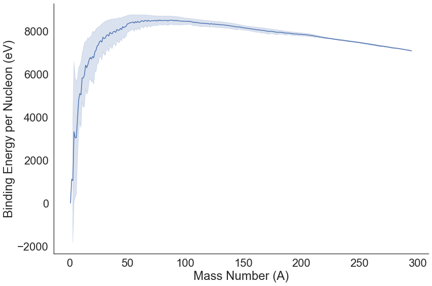
Binding Energy per Nucleon
We can easily plot the binding energy per nucleon using seaborn:
[20]:
sns.relplot(x="A", y="Binding_Energy", kind="line", data=ame, height=8, aspect=1.5, ci="sd")
plt.xlabel("Mass Number (A)")
plt.ylabel("Binding Energy per Nucleon (eV)")
plt.savefig(os.path.join(fig_dir, "AME_BE_per_A.png"), bbox_inches='tight', dpi=500)
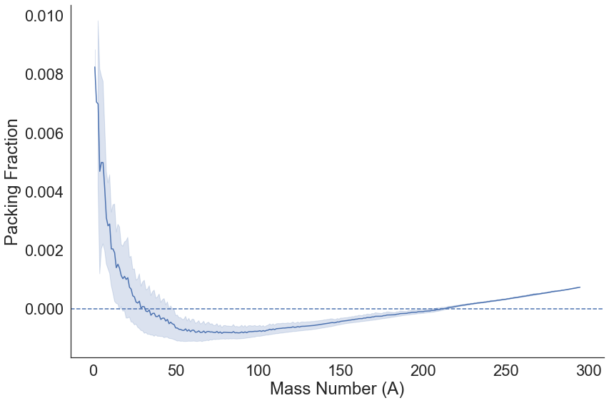
Packing Fraction
[23]:
ame["packing_fraction"] = ((ame.Atomic_Mass_Micro/1E6) - ame.A) / ame.A
[24]:
g = sns.relplot(x="A", y="packing_fraction", kind="line", data=ame, height=8, aspect=1.5, ci="sd")
plt.xlabel("Mass Number (A)")
plt.ylabel("Packing Fraction")
g.axes[0][0].axhline(0, ls='--')
plt.savefig(os.path.join(fig_dir, "AME_packing_fraction.png"), bbox_inches='tight', dpi=500)
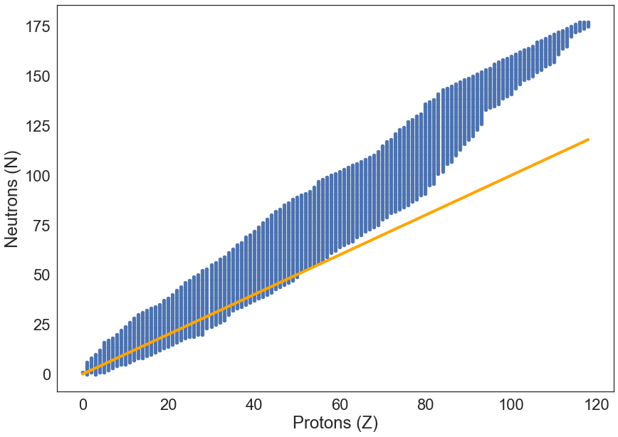
Proton-Neutron Behaviour
[25]:
plt.figure(figsize=(14,10))
ame.plot(x="Z", y="N", kind='scatter', figsize=(14,10))
plt.plot(ame.Z, ame.Z, linewidth=4, color="orange")
plt.xlabel("Protons (Z)")
plt.ylabel("Neutrons (N)")
plt.savefig(os.path.join(fig_dir, "AME_Z_vs_N.png"), bbox_inches='tight', dpi=500)
WARNING:matplotlib.axes._axes:*c* argument looks like a single numeric RGB or RGBA sequence, which should be avoided as value-mapping will have precedence in case its length matches with *x* & *y*. Please use the *color* keyword-argument or provide a 2-D array with a single row if you intend to specify the same RGB or RGBA value for all points.
<Figure size 1008x720 with 0 Axes>
Original vs Imputed AME Dataset
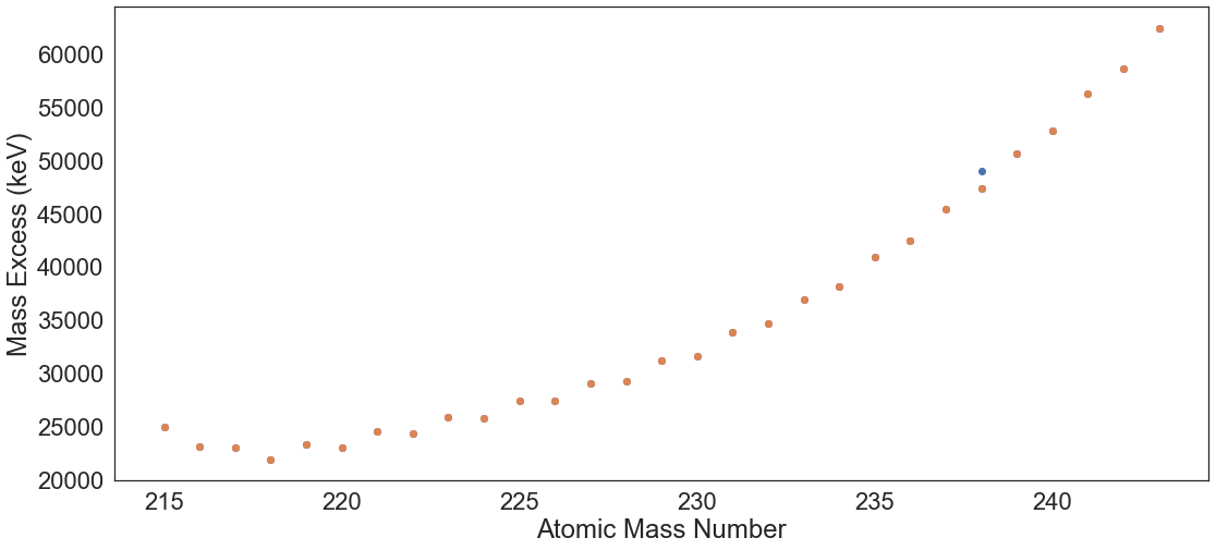
As mentioned in the loading data section of the documentation, the values for the imputed version of the AME dataset were obtained by linear interpolation. We can visualize the imputed values by overlapping both the AME dataset with and without NaN values. For example, let us visualize the Mass Excess value for natural uranium (remember that we needed natural data for EXFOR’s natural target samples):
[27]:
plt.figure(figsize=(18,8))

plt.scatter(ame_filled[ame_filled.Z == 92].sort_values(by="A").A,
            ame_filled[ame_filled.Z == 92].sort_values(by="A").Mass_Excess)
plt.scatter(ame[ame.Z == 92].sort_values(by="A").A,
            ame[ame.Z == 92].sort_values(by="A").Mass_Excess)
plt.ylabel("Mass Excess (keV)")
plt.xlabel("Atomic Mass Number")
[27]:
Text(0.5, 0, 'Atomic Mass Number')
We can automate the creation of these plots:
[28]:
def plot_comparison(protons, feature, ax=None):
    if ax is None:
        ax = plt.gca()
    ax.scatter(ame_filled[ame_filled.Z == protons].sort_values(by="A").A,
             ame_filled[ame_filled.Z == protons].sort_values(by="A")[feature])
    ax.scatter(ame[ame.Z == protons].sort_values(by="A").A,
             ame[ame.Z == protons].sort_values(by="A")[feature])
    ax.set_ylabel(feature.replace("_" ," "))
#     ax.set_xlabel("Atomic Mass Number")
In the following plots, the blue points represent the imputed values either for a natural data point or an isotope for which a value was not reported. In some cases, these values are not applicable but imputation is necessary for compatibility with some ML models. Let us plot the Mass Excess, Binding Energy, Beta Decay Energy, and the Neutron Separation Energy, all in a subplot
[29]:
# make figure with subplots
f, ((ax1, ax2), (ax3, ax4)) = plt.subplots(2, 2, sharex=False, figsize=(25,14))
plot_comparison(92, "Mass_Excess", ax1)
plot_comparison(92, "B_Decay_Energy", ax2)
plot_comparison(92, "Binding_Energy", ax3)
plot_comparison(92, "S(n)", ax4)

ax1.set_xlabel("Atomic Mass Number")
ax2.set_xlabel("Atomic Mass Number")
ax3.set_xlabel("Atomic Mass Number")
ax4.set_xlabel("Atomic Mass Number")

f.savefig(os.path.join(fig_dir, "AME_NaN.png"), bbox_inches='tight', dpi=500)
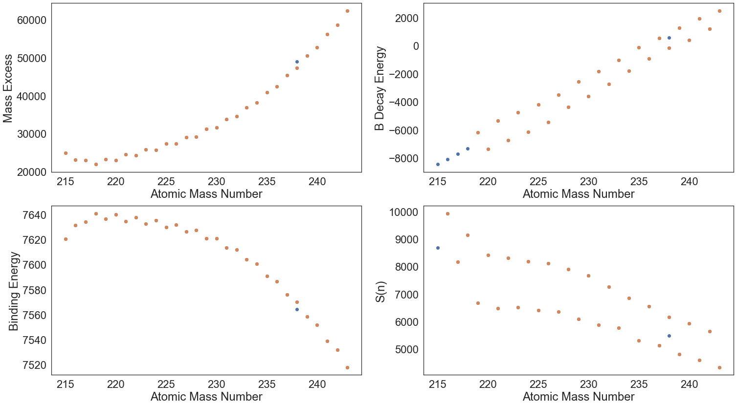
While not perfect, it is better than not using the AME database at all. The AME database contains very useful information that a model can leverage to make better predictions.